Neural Networks Explained: A Visual Guide
SkillVeris Team
Data Science Team
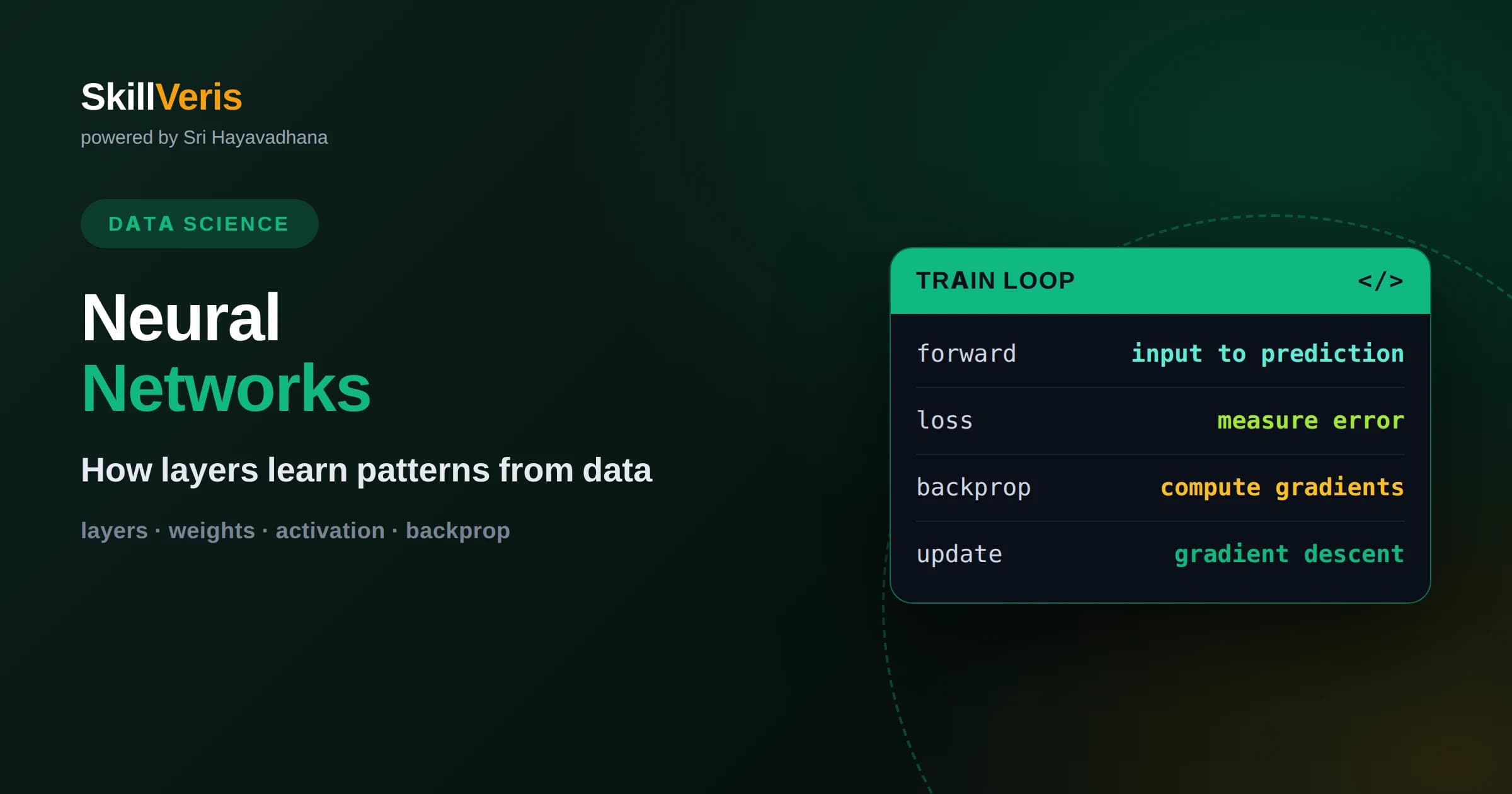
A neural network is a stack of layers of simple units that transform inputs into outputs by multiplying, adding, and applying a nonlinear activation.
In this guide, you'll learn:
- Learning happens through forward propagation to make a prediction, a loss function to measure error, and backpropagation with gradient descent to adjust weights.
- Nonlinear activation functions are what let networks model complex, curved relationships that a plain linear model never could.
- Depth lets networks build features hierarchically, but it also introduces challenges like vanishing gradients and overfitting that practical techniques address.
1What Is A Neural Network
A neural network is a machine learning model that learns patterns by passing data through layers of interconnected units, each of which multiplies its inputs by adjustable weights, adds them up, and applies a simple nonlinear function. By tuning those weights during training, the network gradually learns to map inputs, like the pixels of an image, to outputs, like the label cat or dog. Nothing about the individual pieces is complicated; the power comes from stacking many of them and letting the data set the weights.
The design is loosely inspired by the brain, where neurons fire and pass signals to other neurons. In an artificial network each unit is a tiny math function rather than a biological cell, but the metaphor is useful: signals flow forward through connections, and the strength of each connection, its weight, determines how much influence one unit has on the next.
It helps to picture the network as a series of layers drawn left to right. Data enters at the input layer, flows through one or more hidden layers that transform it, and exits at the output layer as a prediction. Understanding that flow, and how the weights along it are learned, is the whole game.
2The Neuron: The Basic Building Block
A single artificial neuron does three things. It takes several numbers as input, multiplies each by its own weight, and sums the results along with an extra constant called a bias. The bias lets the neuron shift its output up or down independently of the inputs, giving it more flexibility. So far this is just a weighted sum, which is a straight line in disguise.
The crucial fourth step is the activation function, which takes that weighted sum and bends it through a nonlinear curve. Without this bend, no matter how many neurons you stack, the whole network would collapse into a single linear equation, unable to model anything curved or complex. The activation is what gives a neuron the ability to say something more nuanced than a simple proportional response.
Picture the neuron as a small decision gate. It gathers evidence from its inputs, weighs each piece by how much it trusts it, adds a baseline lean from the bias, and then passes the result through a function that decides how strongly to fire. Thousands of these gates working together can represent astonishingly rich patterns.
3Layers And Network Architecture
Neurons are organized into layers. The input layer simply holds your raw features, one unit per feature. Hidden layers sit in the middle and do the real transforming, each one taking the previous layer's outputs and producing a new, more abstract representation. The output layer produces the final answer, with its shape chosen to match the task: one unit for a yes-or-no prediction, or several units for choosing among many categories.
In a fully connected network, every unit in one layer connects to every unit in the next, and each connection carries its own weight. Adding more units per layer widens the network, giving it more capacity in that stage, while adding more layers deepens it, letting it build features in stages.
Depth is where the term deep learning comes from. Early layers tend to learn simple patterns, such as edges in an image, while later layers combine those into more complex concepts, such as shapes and eventually objects. This hierarchical build-up of features, learned automatically from data, is what makes deep networks so powerful on hard problems.
4Activation Functions And Why They Matter
Activation functions are the nonlinear ingredient that makes networks expressive. The most common choice in hidden layers is the rectified linear unit, or ReLU, which passes positive values through unchanged and clips negatives to zero. It is simple, fast, and works well in deep networks, which is why it became the default.
Other functions serve specific roles. The sigmoid squashes any number into a range between zero and one, which is handy for producing a probability at the output of a binary classifier. The softmax function generalizes this to many categories, turning a set of scores into probabilities that add up to one. Choosing the right activation for each layer, especially the output layer, is a small decision with a big effect on whether the network can express what you need.
5Forward Propagation: Making A Prediction
Forward propagation is the process of pushing an input through the network to get an output. Each layer takes the numbers from the previous layer, applies its weights, biases, and activation, and hands the result to the next layer. By the time the data reaches the output layer, it has been transformed step by step into a prediction.
At first, with random initial weights, these predictions are essentially guesses. The point of forward propagation is not that it starts out accurate but that it is repeatable and measurable. Because every step is a clear mathematical operation, we can later trace exactly how each weight contributed to the final answer, which is what makes learning possible.
Forward propagation is also what happens at prediction time, once the network is trained. The very same flow that produces guesses during early training produces trustworthy answers on new data after the weights have been tuned. In other words, training and inference share the same forward machinery; training simply wraps it in a loop that keeps adjusting the weights until those forward passes come out right.
6Measuring Error With A Loss Function
To improve, a network needs a way to score how wrong it is. That is the job of the loss function, which compares the network's prediction to the true answer and outputs a single number representing the error. A large loss means the prediction was far off; a loss near zero means it was nearly perfect.
Different tasks call for different losses. For predicting a continuous quantity, mean squared error, which averages the squared gaps between predictions and truth, is a natural choice. For classification, cross-entropy loss measures how far the predicted probabilities stray from the correct category. Whatever the task, the loss turns the vague goal of being accurate into a precise number the network can try to shrink.
7Backpropagation: How Networks Learn
Backpropagation is the algorithm that assigns blame for the error to each weight in the network. After forward propagation produces a prediction and the loss measures the error, backpropagation works backward from the output, using the chain rule of calculus to compute how much each weight contributed to the loss. The result is a gradient, a direction telling each weight whether to increase or decrease to reduce the error.
The name captures the flow: information about the error propagates backward through the same connections the data flowed forward along. Weights near the output get updated based on their direct effect, and that signal is passed further back so that deeper weights learn too. Backpropagation is efficient because it reuses intermediate calculations rather than recomputing everything for each weight.
It is worth stressing that backpropagation only computes the gradients. It says which way to nudge each weight; a separate step actually performs the nudge. Keeping those two roles distinct makes the whole learning process easier to reason about.
8Gradient Descent And Learning Rate
Gradient descent is the step that uses the gradients to update the weights. Each weight moves a small amount in the direction that reduces the loss, and the size of that step is controlled by the learning rate. Repeat forward propagation, loss, backpropagation, and a gradient descent update many times, and the network slowly walks its way toward weights that make good predictions.
The learning rate is a delicate dial. Too large and the updates overshoot, bouncing around or even diverging so the loss grows instead of shrinking. Too small and training crawls, taking far too many steps to improve. In practice, networks are trained in mini-batches, updating weights after each small group of examples, which balances speed and stability. Modern optimizers automatically adapt the effective step size to make this tuning less fragile.
9The Training Loop In Full
Put the pieces together and you have the training loop. Feed a batch of examples forward to get predictions, compute the loss against the true answers, run backpropagation to get the gradients, and apply a gradient descent update to the weights. Then repeat with the next batch. One full pass through the entire dataset is called an epoch, and networks usually train for many epochs.
Over time, if all goes well, the loss trends downward and the predictions improve. Watching the loss curve is one of the most informative habits in deep learning: a steadily falling loss suggests healthy learning, while a flat or erratic curve hints at a learning rate problem, a data issue, or an architecture that is a poor fit for the task.
10Overfitting And How To Prevent It
Because neural networks have so many weights, they can memorize the training data instead of learning general patterns, a failure called overfitting. An overfit network performs beautifully on data it has seen and poorly on anything new, which defeats the purpose. Watching the gap between training performance and validation performance is how you catch it.
Several techniques keep networks honest. Dropout randomly switches off some units during training so the network cannot rely on any single path and must learn redundant, robust features. Weight regularization penalizes overly large weights, nudging the model toward simpler solutions. And early stopping halts training once validation performance stops improving, before the network starts memorizing. Used together, these tools help a network generalize rather than merely remember.
11Common Network Architectures
The basic fully connected network is only the beginning. Convolutional neural networks are designed for images; they slide small filters across the picture to detect local patterns like edges and textures, sharing weights so they need far fewer parameters and respect the spatial structure of an image. Recurrent networks were built for sequences, feeding their own output back as input so they can carry context from earlier steps to later ones.
Transformers, which now dominate language and increasingly other domains, use a mechanism called attention to let every part of the input weigh the relevance of every other part directly. Each of these architectures is still built from the same fundamentals: weighted sums, activations, a loss, and backpropagation. Learning the fundamentals first makes every specialized architecture far easier to understand later.
12Why Neural Networks Work So Well
Neural networks excel because they learn their own features. Traditional models often depend on humans to hand-craft the right input features, which is slow and limited. A deep network instead discovers useful features automatically, layer by layer, directly from raw data, which is why they have driven breakthroughs in vision, language, and speech.
This power comes with costs. Networks are data-hungry, computationally expensive to train, and harder to interpret than simpler models, since the learned patterns are spread across thousands of weights. Knowing both the strengths and the trade-offs lets you choose a neural network when it genuinely fits the problem rather than reaching for one by reflex.
13Start Building Your Own Networks
The concepts click into place the moment you build a small network and watch it learn. Begin with a tiny network on a simple dataset, print the loss each epoch, and change one thing at a time: the learning rate, the number of hidden units, the activation function. Seeing how each change moves the loss curve builds intuition that no amount of reading can replace.
On SkillVeris you can follow guided lessons that take you from a single neuron to a full training loop, with exercises that let you experiment safely and see results immediately. Working through these hands-on, and getting comfortable with the forward pass, the loss, and backpropagation, gives you a foundation strong enough to understand any modern architecture you meet later.
Related Reading
Get The Print Version
Download a PDF of this article for offline reading.
About the Publisher
SkillVeris Team
Data Science Team
Our data team shares real-world analytics, ML, and SQL insights grounded in industry practice.
View all postsRelated Posts

Never miss an update
Get the latest tutorials and guides delivered to your inbox.
No spam. Unsubscribe anytime.