Linear Regression Explained From Scratch
SkillVeris Team
Data Science Team
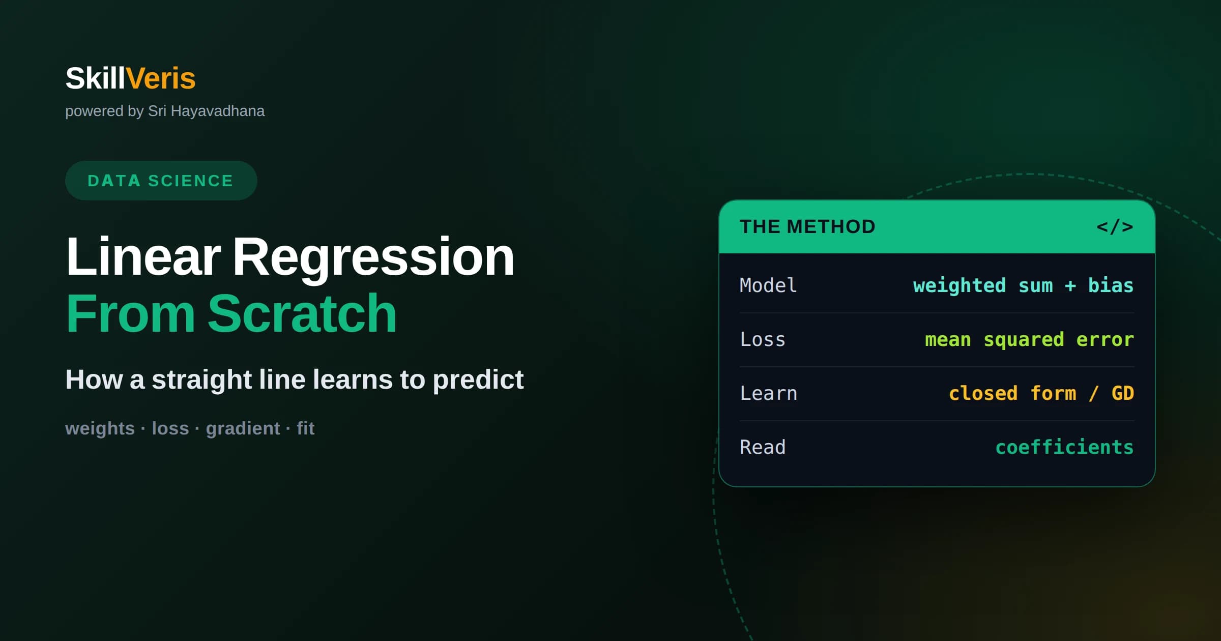
Linear regression predicts a continuous number by fitting a weighted sum of the input features.
In this guide, you'll learn:
- It learns by minimizing the squared difference between its predictions and the true values.
- The coefficients are directly interpretable, telling you how each feature moves the prediction.
- Understanding its assumptions tells you when linear regression works and when it quietly fails.
1What Linear Regression Actually Does
Linear regression is a method for predicting a continuous number by assuming the output is a straight-line, weighted combination of the input features. In its simplest form with one input, it fits the best straight line through a cloud of points so you can estimate the output for any new input. It is the foundational algorithm of predictive modeling and the natural first thing to learn.
The word linear means the model combines inputs additively, each scaled by its own weight, with no curves or interactions unless you add them yourself. Despite that simplicity, linear regression is remarkably useful and remains one of the most used models in practice because it is fast, interpretable, and often good enough.
Learning it from scratch, rather than treating it as a black box, pays off because every more advanced method builds on these ideas. Gradient descent, loss functions, overfitting, and regularization all appear here in their clearest form, making linear regression the ideal place to build real understanding. When you later meet a neural network, you will recognize that each of its units is essentially a small linear regression with a twist, so the effort you invest here keeps paying dividends.
2The Model as a Weighted Sum
The prediction is a weighted sum of the inputs plus a constant. Each feature has a coefficient, sometimes called a weight, that says how much that feature contributes, and there is an intercept term that sets the baseline when all features are zero. Together these numbers define the line, or in higher dimensions the plane, that the model uses.
With a single input, the equation is the familiar line: the prediction equals a slope times the input plus an intercept. The slope tells you how much the output changes for each one-unit increase in the input, and the intercept tells you where the line crosses when the input is zero.
With many inputs, the same idea generalizes: each feature gets its own slope, and the prediction is the sum of all these contributions plus the intercept. The whole model is nothing more than these coefficients, which is why linear regression is so easy to inspect and explain.
3Measuring How Wrong the Line Is
To fit the best line, you first need a way to measure how bad any given line is. Linear regression uses the squared error: for each data point, take the difference between the prediction and the true value, square it, and sum across all points. This total is called the loss, and smaller is better.
Squaring the errors serves two purposes. It makes all errors positive so they do not cancel out, and it penalizes large mistakes much more heavily than small ones. A prediction that is off by four contributes sixteen to the loss, while one off by two contributes only four, so the model works hard to avoid big misses.
The average of these squared errors is the mean squared error, one of the most common metrics in all of machine learning. Minimizing it is exactly what fitting a linear regression means, so this simple quantity sits at the center of everything the algorithm does.
4Finding the Best-Fit Line
Fitting the model means finding the coefficients that make the total squared error as small as possible. Remarkably, for linear regression there is an exact mathematical formula, derived with calculus, that computes the optimal coefficients directly. This closed-form solution is why linear regression trains almost instantly on modest datasets.
The idea behind the formula is that at the minimum of the loss, the slope of the loss with respect to each coefficient is zero. Setting those slopes to zero and solving gives the unique best answer. You do not need to derive it by hand to use it, but knowing it exists explains why the model is so fast and reliable.
This exactness is special. Most machine learning models have no closed-form solution and must be trained by iterative search. Linear regression is a rare case where the mathematics hands you the perfect answer in one step, which makes it a clarifying example to study first.
5Learning by Gradient Descent
Even though a formula exists, it is worth understanding the iterative alternative called gradient descent, because it is how nearly every larger model learns. Gradient descent starts with random coefficients and repeatedly nudges them in the direction that reduces the loss a little, taking many small steps toward the minimum.
The gradient is the direction of steepest increase in the loss, so moving in the opposite direction decreases it. A setting called the learning rate controls how big each step is. Too large and the steps overshoot and diverge; too small and training crawls. Choosing it well is a skill you will use with every gradient-based model.
Watching gradient descent converge on the same answer the formula gives is a powerful way to build intuition. It shows that learning is just repeated, informed improvement, and that same principle scales up to models with millions of parameters where no formula exists.
6Interpreting the Coefficients
One of linear regression's greatest strengths is that its coefficients mean something. Each coefficient tells you how much the prediction changes when its feature increases by one unit, holding the other features fixed. This direct interpretability is why the model is trusted in fields like economics and medicine where understanding matters as much as accuracy.
The sign of a coefficient tells you the direction of the relationship: positive means the output rises with the feature, negative means it falls. The magnitude tells you the strength, though you must account for the scale of each feature, which is why standardizing inputs makes coefficients more comparable.
Be careful not to read causation into these numbers. A coefficient describes association within your data, not proof that changing the feature would change the outcome. Confounding variables can create relationships that vanish once you account for them, so interpret with humility.
7The Assumptions Behind the Method
Linear regression works best when certain assumptions hold. It assumes the true relationship is roughly linear, that the errors have constant spread across the range of predictions, that the errors are independent, and that they are roughly normally distributed. When these hold, the model's estimates and confidence in them are trustworthy.
In practice these assumptions are never perfectly met, and mild violations are usually fine. The point of knowing them is to recognize serious violations that break the model. If the true relationship curves sharply, a straight line will fit poorly no matter how you train it.
Diagnostic plots of the residuals, the leftover errors after fitting, are how you check these assumptions. A random, patternless cloud of residuals is healthy; visible curves or funnels signal that an assumption is violated and the model needs rethinking.
8Overfitting and Regularization
Even a simple model can overfit when you have many features relative to the amount of data. Overfitting means the model learns noise specific to the training set and then generalizes poorly. In linear regression this often shows up as wildly large coefficients that fit the training points too precisely.
Regularization tames this by adding a penalty for large coefficients to the loss. Two common forms are ridge regression, which shrinks coefficients smoothly, and lasso regression, which can shrink some all the way to zero and thereby select features. Both trade a little training accuracy for better generalization.
Regularization introduces a tuning knob that balances fitting the data against keeping the model simple. Setting it well requires validation on held-out data, and it is your first encounter with the pervasive trade-off between bias and variance that runs through all of machine learning.
9Preparing Features for Linear Regression
Linear regression only sees the features you give it, so preparation matters. Categorical variables must be encoded into numbers, and features on very different scales should often be standardized, especially when using regularization, so the penalty applies fairly across them.
Because the model is strictly linear, you can capture curved relationships only by engineering features that express them, such as adding a squared term or a ratio. This manual feature engineering is how a linear model can fit surprisingly complex patterns while keeping its interpretable structure.
Watch for features that are highly correlated with each other, a condition called multicollinearity. It makes coefficients unstable and hard to interpret, because the model cannot tell which of the correlated features deserves the credit. Removing or combining such features usually helps.
10When to Use Linear Regression
Reach for linear regression when your target is a continuous number and you want a fast, interpretable baseline. It shines when the relationship is roughly linear and when explaining the model to stakeholders is as important as raw accuracy. In many business settings that combination is exactly what is needed.
It is also the right first model on almost any regression problem, even when you expect to end up with something more complex. The baseline it provides tells you whether fancier models are actually adding value, which protects you from over-engineering.
Where relationships are strongly nonlinear or involve rich interactions you cannot easily engineer, tree-based models or neural networks may do better. But even then, understanding linear regression makes those advanced methods far easier to grasp.
11Putting the Pieces Together
Step back and the whole method is a tidy loop. You propose a weighted-sum model, measure its error with mean squared error, and find the coefficients that minimize that error either by formula or by gradient descent. You then interpret the coefficients, check the assumptions with residual plots, and regularize if the model overfits.
Every one of those steps reappears in more sophisticated models, often in disguise. The loss function becomes cross-entropy, the closed-form solution disappears, and the linear layer becomes one of many, but the skeleton is identical. That is why time spent truly understanding linear regression compounds throughout your learning.
Once you can explain each step in your own words, you have a foundation that makes classification, deep learning, and beyond noticeably less mysterious. The vocabulary and intuition simply carry over.
12Evaluating How Good the Fit Is
Once you have fit a line, you need to judge how well it explains the data. Mean squared error and its square root, the root mean squared error, report the typical size of the prediction errors in the units of the target, which makes them easy to communicate to non-specialists.
A complementary measure is the coefficient of determination, often written as R squared, which reports the fraction of the variation in the target that the model explains. A value near one means the line captures most of the pattern, while a value near zero means it explains little more than simply guessing the average.
Always compute these metrics on held-out data, never on the data the model was fit to. A model can score well on its training set and still fail on new inputs, so an honest evaluation on unseen data is the only trustworthy measure of how the model will actually perform.
13Practice Linear Regression on SkillVeris
The best way to cement these ideas is to implement linear regression yourself and then compare your version to a library implementation on the same data. Building the loss, running gradient descent, and watching it converge turns abstract formulas into something you genuinely understand rather than merely recognize.
SkillVeris offers guided, hands-on lessons that walk you through both the from-scratch mechanics and the practical library workflow, then connect linear regression to the classification and regularization topics that build on it. Working through them gives you the deep, transferable understanding that makes everything after linear regression easier.
Related Reading
Get The Print Version
Download a PDF of this article for offline reading.
About the Publisher
SkillVeris Team
Data Science Team
Our data team shares real-world analytics, ML, and SQL insights grounded in industry practice.
View all postsRelated Posts


Never miss an update
Get the latest tutorials and guides delivered to your inbox.
No spam. Unsubscribe anytime.