Big-O Notation Explained: Time & Space Complexity
SkillVeris Team
Engineering Team
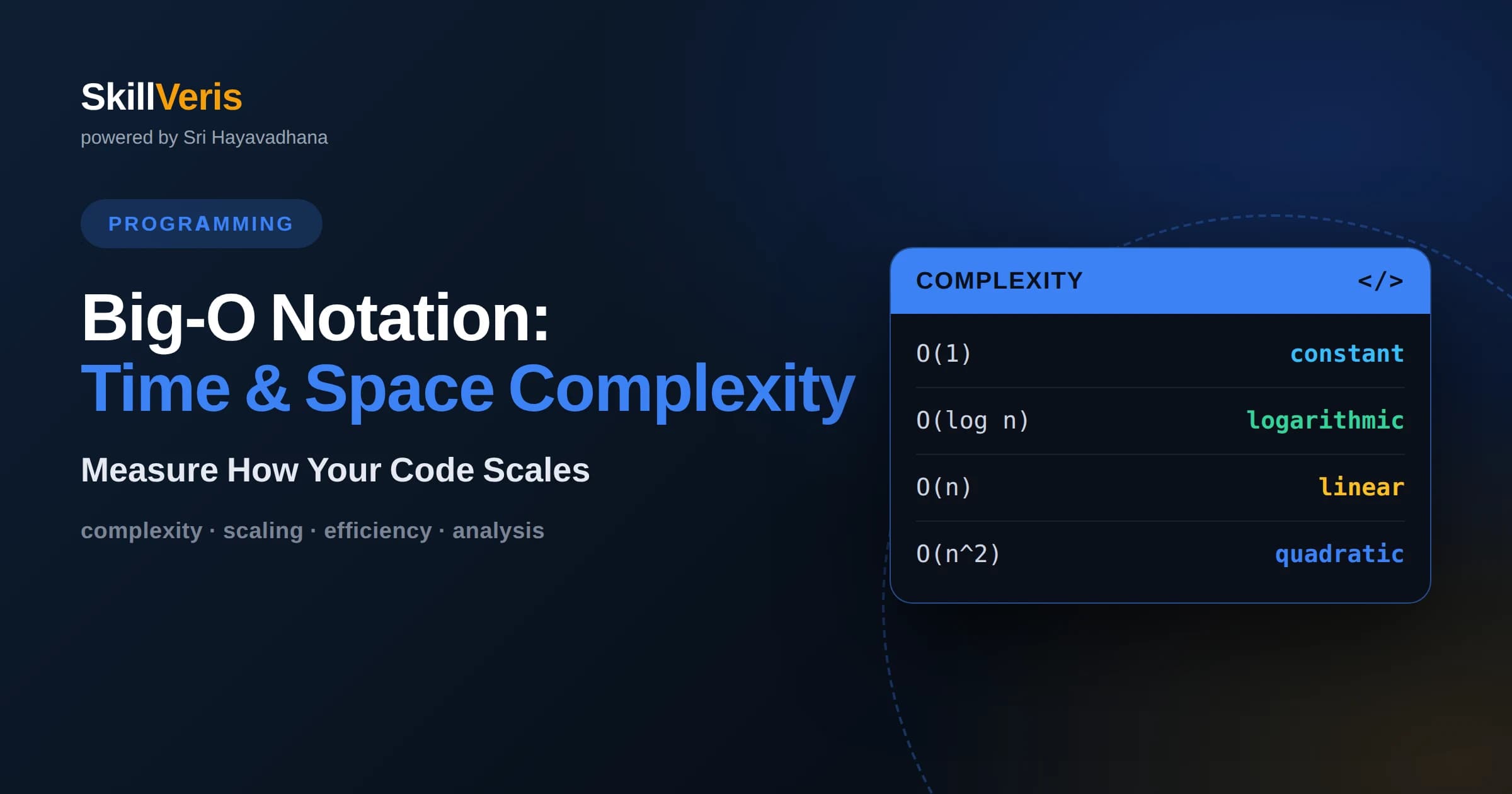
Big-O notation describes how an algorithm's running time or memory grows as the input size grows, letting you compare algorithms independently of hardware or language.
In this guide, you'll learn:
- The common complexity classes from fastest to slowest are constant, logarithmic, linear, linearithmic, quadratic, and exponential, and recognizing them on sight is a core interview skill.
- Big-O focuses on the dominant term and ignores constants, so 2n plus 100 and 5n both simplify to O(n) because they scale the same way at large input sizes.
- Space complexity measures extra memory an algorithm uses beyond its input, and a good engineer weighs time and space trade-offs rather than optimizing one blindly.
1What Big-O Notation Actually Means
Big-O notation is a way of describing how the resources an algorithm needs grow as the size of its input grows. When we say an algorithm is O(n), we mean that if you double the input, the work roughly doubles too. It is a language for talking about scalability, not about exact seconds on a particular machine.
This distinction is what makes Big-O so useful. A fast laptop can run a badly designed algorithm quickly on small inputs, hiding the problem until the data grows. Big-O cuts through that by describing the growth pattern itself, so you can predict behavior on a million items after testing on only a few hundred.
The letter O stands for order of growth, and the expression inside the parentheses captures how the cost scales with the input size, usually called n. Throughout this article we will build up an intuition for the common orders of growth and how to spot them in real code.
2Why Big-O Matters
Every non-trivial program eventually meets a large input, and the difference between a fast algorithm and a slow one becomes brutal at scale. An O(n) approach on a million items does about a million operations, while an O(n squared) approach does a trillion. On the same hardware, one finishes instantly and the other appears to hang forever.
Big-O gives you a vocabulary to make these trade-offs before you write a line of code. Instead of guessing, you can reason that a nested loop over the same data will scale quadratically and look for a smarter approach. This kind of upfront analysis is what separates code that survives growth from code that collapses under it.
It also matters because interviewers lean on it heavily. When you are asked to solve a coding problem, the follow-up is almost always about the time and space complexity of your solution. Being fluent in Big-O signals that you can reason about performance, which is a core expectation for any serious engineering role.
3How to Read and Simplify Big-O
Big-O follows two simplifying rules that make it practical. First, you drop constant factors, so an algorithm that does 5n operations and one that does 100n operations are both O(n), because they scale the same way as n grows. Constants matter in the real world but not in the growth classification.
Second, you keep only the dominant term. If an algorithm does n squared plus n operations, the n squared term utterly dominates as n grows large, so we write O(n squared) and discard the smaller term. Big-O describes behavior at scale, where the biggest term drowns out everything else.
Put together, an expression like 3n squared plus 10n plus 50 simplifies to O(n squared). This might feel like throwing away information, but that is the point: Big-O deliberately zooms out to the shape of the growth curve, which is exactly what you need when comparing how algorithms behave on large inputs.
4Constant Time: O(1)
An operation is O(1), or constant time, when it takes the same amount of work regardless of input size. Accessing an element in an array by its index, like grabbing numbers[5], is constant time because the computer can jump straight to that memory location without scanning anything.
Constant time is the gold standard, but it does not mean instant or free; it means the cost does not grow with the input. Looking up a value in a hash map or dictionary by its key is typically O(1) on average, which is why dictionaries are such a beloved tool for fast lookups.
When you see a solution that turns a slow search into a single dictionary lookup, you are often watching an algorithm move from linear time down to constant time for that step. Recognizing opportunities to trade a little memory for constant-time lookups is one of the most useful practical skills in algorithm design.
5Linear Time: O(n)
Linear time, written O(n), means the work grows in direct proportion to the input. A single loop that visits every item once, such as summing all the numbers in a list, is the classic example. Double the list and you do double the work, which is a fair and often unavoidable cost.
Many everyday tasks are inherently linear because you simply must look at every element at least once. Finding the maximum value in an unsorted list, counting how many items match a condition, or printing every record all require touching each item, and no clever trick can beat O(n) when every element genuinely matters.
Linear time is usually considered efficient and acceptable. The important skill is recognizing when your code is accidentally worse than linear, for example when a loop hides another loop inside it, quietly turning an O(n) task into something far more expensive.
6Logarithmic Time: O(log n)
Logarithmic time, O(log n), describes algorithms that cut the problem roughly in half at each step. The signature example is binary search on a sorted list: you check the middle element, decide whether your target is in the left or right half, and discard the other half entirely. Each comparison eliminates half of what remains.
This halving is astonishingly powerful. Searching a sorted list of a billion items takes only about thirty comparisons, because you keep halving until one item is left. That is why logarithmic algorithms feel almost free even on enormous inputs, and why keeping data sorted or in balanced trees is so valuable.
The catch is that logarithmic search usually requires structure, such as a sorted array or a balanced tree, which itself has a cost to build and maintain. The trade-off is often worth it when you search the same data many times, because you pay the setup cost once and enjoy fast lookups repeatedly.
7Linearithmic Time: O(n log n)
O(n log n), sometimes called linearithmic time, is the complexity of the best general-purpose sorting algorithms like merge sort and the sorts built into most standard libraries. It sits between linear and quadratic, and for sorting it is provably the best you can do with comparison-based methods.
Intuitively, you can think of merge sort as repeatedly splitting the data in half, which contributes the log n factor, and then doing linear work to merge the pieces back together at each level, which contributes the n factor. Multiply them and you get n log n.
Whenever a problem involves sorting as a step, you should expect at least O(n log n) for that part. Recognizing this helps you set realistic expectations: if your overall algorithm sorts the data and then does a linear pass, the sort dominates and the whole thing is O(n log n).
8Quadratic Time: O(n squared)
Quadratic time, O(n squared), appears whenever you have a loop inside a loop, each running over the input. Comparing every item to every other item, as in a naive approach to finding duplicate pairs, does roughly n times n operations. On small inputs this is fine, but the cost explodes quickly.
The danger of quadratic algorithms is how innocent they look. A pair of nested loops is easy to write and reads perfectly well, yet on ten thousand items it performs a hundred million operations. Many performance disasters trace back to an accidental nested loop that no one noticed while the test data was tiny.
The good news is that quadratic solutions can often be improved. Sorting the data first, or using a hash map to remember what you have already seen, frequently drops an O(n squared) approach down to O(n log n) or even O(n). Spotting the nested-loop pattern is the first step toward that optimization.
9Exponential and Factorial Time
Exponential time, O(2 to the n), and factorial time, O(n factorial), are the danger zone. They arise in brute-force solutions to problems like generating every subset of a set or trying every possible arrangement of items. The cost roughly doubles or worse with each additional element, so even modest inputs become impossible.
To feel the scale, an exponential algorithm on just fifty items may require more operations than there are atoms in a visible region of the universe. These complexities are not merely slow; they are fundamentally infeasible beyond tiny inputs, which is why they signal that a smarter strategy is required.
Encountering exponential complexity is often a hint to reach for techniques like dynamic programming, greedy strategies, or clever pruning that avoid re-exploring the same work. Recognizing that a naive recursive solution is exponential is exactly the insight interviewers hope you will voice before optimizing.
10Space Complexity
Space complexity measures how much extra memory an algorithm uses as the input grows, beyond the space taken by the input itself. An algorithm that scans a list and keeps only a running total uses O(1) extra space, while one that builds a new list of the same size uses O(n) extra space.
Time and space often trade against each other. Caching results or building a lookup table can turn a slow computation into a fast one, but it costs memory. Conversely, an algorithm that recomputes values to save memory may run slower. A thoughtful engineer weighs both dimensions rather than fixating on speed alone.
Recursion deserves special attention because each nested call adds a frame to the call stack, consuming memory even if the code creates no new data structures. A deep recursion can be O(n) in space just from the stack, which is easy to overlook when you are focused only on running time.
11Best, Worst, and Average Cases
Big-O most often describes the worst case, the upper bound on how slow an algorithm can get, because that is what protects you from unpleasant surprises. But algorithms also have best and average cases, and knowing the difference sharpens your reasoning about real performance.
Consider searching an unsorted list for a value. In the best case the item is first, giving O(1); in the worst case it is last or missing, giving O(n); and on average you scan about half the list, which is still O(n) after dropping the constant. The worst case governs the guarantee you can make.
Some algorithms have a great average case but a rare bad worst case, which matters when you need dependable performance under adversarial conditions. Being able to discuss best, worst, and average complexity shows a level of maturity that stands out in technical interviews and in real engineering decisions.
12A Worked Example: Finding Duplicates
Suppose you must decide whether a list contains any duplicate values. The naive approach compares every element to every other element using two nested loops. For each item you scan the rest of the list, which gives O(n squared) time and only O(1) extra space, since you store nothing new.
A faster approach uses a set to remember values you have already seen. You loop once through the list, and for each item you check whether it is already in the set. Membership checks in a set are O(1) on average, so the whole scan becomes O(n) time. The cost is O(n) extra space to hold the set.
This single example captures the heart of Big-O thinking: the second solution trades memory for speed, dropping from quadratic to linear time by spending linear extra space. Being able to articulate that trade-off out loud, and to justify which side is worth it for a given situation, is precisely the reasoning that interviews are designed to surface.
13How to Master Big-O on SkillVeris
Big-O clicks fastest when you tie the abstract growth curves to something concrete, which is exactly how SkillVeris teaches it. Its data structures and algorithms track explains each complexity class through a hobby you already understand, so ideas like halving a search space or nesting loops map onto familiar activities and become intuitive rather than intimidating.
The most effective way to internalize complexity analysis is to practice classifying real code. As you work through algorithm lessons, pause on each solution and name its time and space complexity before checking the answer, then look for a version that improves one of them. That habit builds the instant recognition interviewers reward.
Pair the algorithms material with the interview-preparation resources to rehearse explaining your analysis under pressure, and with the broader programming and Python courses to keep your coding sharp. Because SkillVeris is free and personalized, you can move from understanding Big-O to confidently applying it across dozens of practice problems at your own pace.
Get The Print Version
Download a PDF of this article for offline reading.
About the Publisher
SkillVeris Team
Engineering Team
Our engineering writers turn abstract code concepts into hands-on, project-driven learning experiences.
View all postsRelated Posts
Never miss an update
Get the latest tutorials and guides delivered to your inbox.
No spam. Unsubscribe anytime.