Scikit-Learn for Beginners: Machine Learning in Python

SkillVeris Team

Data Science Team

May 8, 2026 11 min read

Scikit-Learn for Beginners: Machine Learning in Python

Key Takeaway

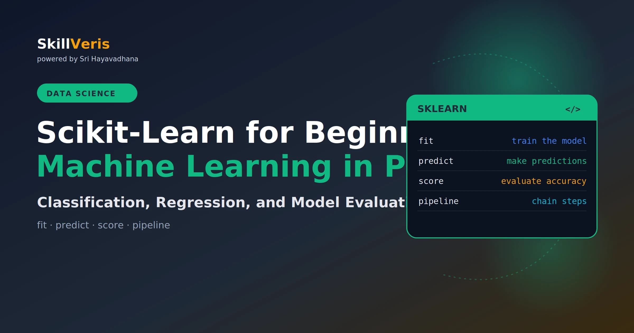
Scikit-learn's API is elegantly consistent: every model has fit(X, y), predict(X), and score(X, y).

In this guide, you'll learn:

Train on training data, evaluate on test data, and use cross-validation for reliable performance estimates.
Switching algorithms is just changing the class name — the rest of the code stays the same.
Always split train/test before any preprocessing, and fit scalers on the training data only to avoid data leakage.
For imbalanced classes use precision, recall, F1, and ROC-AUC instead of accuracy; for regression use RMSE, MAE, and R2.

1What Is Scikit-Learn?

Scikit-learn (sklearn) is the standard Python library for classical machine learning: linear regression, logistic regression, decision trees, random forests, support vector machines, k-means clustering, and more.

It provides a clean, consistent API that makes switching between algorithms easy, plus excellent tools for model evaluation, preprocessing, and pipeline construction.

Common Imports

A typical set of imports for a sklearn project.

code

import sklearn
print(sklearn.__version__)  # 1.4.x or later
from sklearn.linear_model import LogisticRegression, LinearRegression
from sklearn.tree import DecisionTreeClassifier
from sklearn.ensemble import RandomForestClassifier
from sklearn.model_selection import train_test_split, cross_val_score
from sklearn.metrics import accuracy_score, classification_report
from sklearn.pipeline import Pipeline
from sklearn.preprocessing import StandardScaler, OneHotEncoder

2The Consistent API

Every scikit-learn model follows the same three-method API: fit to train, predict on new data, and score to evaluate. Switching algorithms is just changing the class name — the rest of the code stays the same. This uniformity is sklearn's greatest strength.

The four main ML task types and when to use each.

fit, predict, score

The same three methods work across every estimator.

code

# Create model
model = RandomForestClassifier(n_estimators=100, random_state=42)
# Train on labelled data
model.fit(X_train, y_train)
# Predict on new data
predictions = model.predict(X_test)
# Evaluate
score = model.score(X_test, y_test)  # accuracy for classifiers, R2 for regressors

3Loading and Preparing Data

Scikit-learn ships with built-in datasets for learning, and works seamlessly with pandas DataFrames loaded from CSV. The library expects X with shape (n_samples, n_features) and y with shape (n_samples,).

Loading Built-in and CSV Data

Separate the feature matrix X from the target y.

code

from sklearn.datasets import load_iris, load_diabetes
import pandas as pd
# Built-in datasets for learning
iris = load_iris(as_frame=True)
df = iris.frame
X = iris.data  # feature matrix: (150, 4)
y = iris.target  # labels: 0, 1, 2
# From a CSV
df = pd.read_csv("data.csv")
X = df.drop("target", axis=1)  # all columns except target
y = df["target"]  # target column
# sklearn expects: X shape (n_samples, n_features), y shape (n_samples,)
print(X.shape, y.shape)  # e.g. (150, 4) (150,)

4Train/Test Split

Never evaluate a model on data it was trained on — that gives optimistically biased results. Always hold out a test set and use it only for final evaluation. The stratify argument preserves class proportions across both splits.

⚠️Watch Out

Data leakage happens when information from the test set influences training. Common causes: fitting preprocessing (StandardScaler, PCA) on all data instead of training data only; including future data in features; target leakage (a feature only known after the target is known). Leakage produces models that look great in evaluation but fail in production.

Splitting the Data

An 80/20 split with a fixed random_state for reproducibility.

code

from sklearn.model_selection import train_test_split
# Split 80% train, 20% test
X_train, X_test, y_train, y_test = train_test_split(
    X, y,
    test_size=0.2,    # 20% for testing
    random_state=42,  # reproducible split
    stratify=y        # preserve class proportions in both splits
)
print(f"Train: {X_train.shape[0]} samples")
print(f"Test: {X_test.shape[0]} samples")

5Classification: Predicting Categories

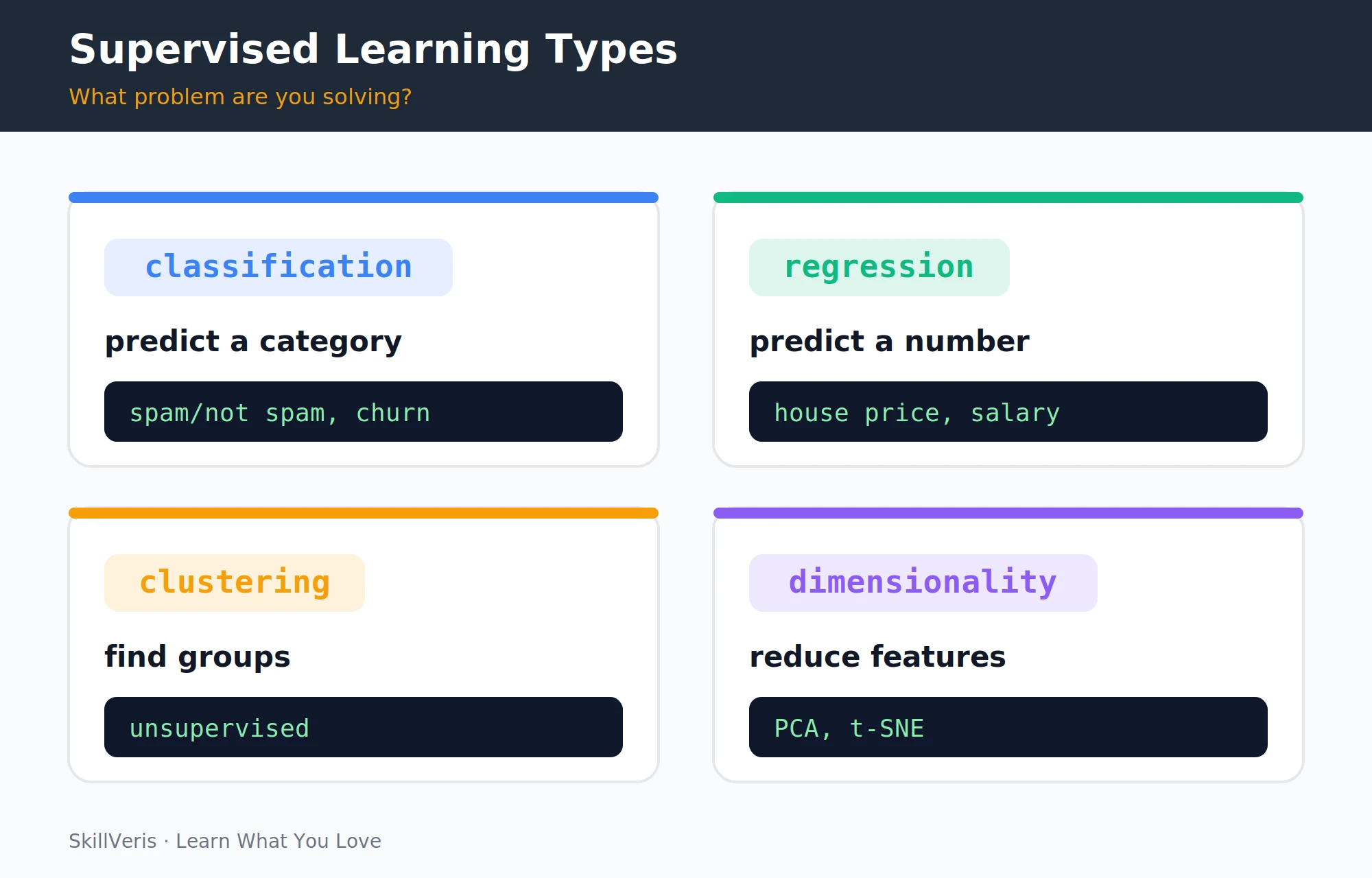
Classification predicts discrete categories. The example below trains a Random Forest on the breast cancer dataset and measures accuracy, which typically lands around 0.96.

A Random Forest Classifier

Fit, predict, and score in a few lines.

code

from sklearn.datasets import load_breast_cancer
from sklearn.ensemble import RandomForestClassifier
from sklearn.model_selection import train_test_split
from sklearn.metrics import accuracy_score
data = load_breast_cancer()
X, y = data.data, data.target
X_train, X_test, y_train, y_test = train_test_split(
    X, y, test_size=0.2, random_state=42, stratify=y)
model = RandomForestClassifier(n_estimators=100, random_state=42)
model.fit(X_train, y_train)
preds = model.predict(X_test)
acc = accuracy_score(y_test, preds)
print(f"Accuracy: {acc:.3f}")  # typically ~0.96

6Model Evaluation for Classification

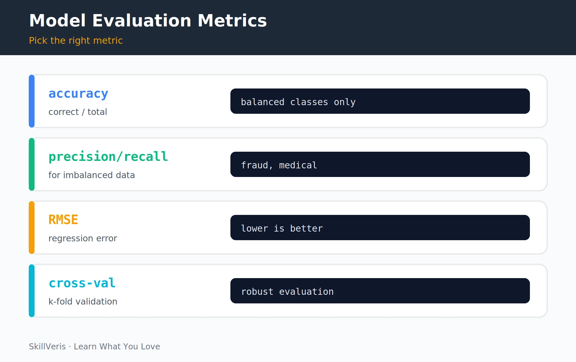
Accuracy alone can mislead. For imbalanced datasets (90% class 0, 10% class 1), a model that always predicts "class 0" gets 90% accuracy. Use precision, recall, F1-score, and ROC-AUC instead, alongside a confusion matrix.

Matching the evaluation metric to the problem type.

Classification Metrics

A full report, confusion matrix, and ROC-AUC.

code

from sklearn.metrics import (classification_report, confusion_matrix,
                             ConfusionMatrixDisplay, roc_auc_score)
# Full classification report
print(classification_report(y_test, preds, target_names=data.target_names))
# Confusion matrix
cm = confusion_matrix(y_test, preds)
disp = ConfusionMatrixDisplay(cm, display_labels=data.target_names)
disp.plot()
# ROC-AUC (for binary classification with probability scores)
proba = model.predict_proba(X_test)[:, 1]  # probability of positive class
auc = roc_auc_score(y_test, proba)
print(f"ROC-AUC: {auc:.3f}")

7Regression: Predicting Numbers

Regression predicts continuous numbers. Ridge adds regularisation to linear regression, while Gradient Boosting is usually the best performer on tabular data.

Ridge and Gradient Boosting

Two regressors on the diabetes dataset.

code

from sklearn.datasets import load_diabetes
from sklearn.linear_model import Ridge
from sklearn.ensemble import GradientBoostingRegressor
data = load_diabetes()
X, y = data.data, data.target
X_train, X_test, y_train, y_test = train_test_split(
    X, y, test_size=0.2, random_state=42)
# Linear regression with regularisation
ridge = Ridge(alpha=1.0)
ridge.fit(X_train, y_train)
# Gradient boosting (usually best for tabular data)
gb = GradientBoostingRegressor(n_estimators=200, learning_rate=0.1, random_state=42)
gb.fit(X_train, y_train)
preds = gb.predict(X_test)

8Model Evaluation for Regression

Regression metrics quantify error in the target's units. RMSE and MAE measure average error, while R2 ranges from 1.0 (perfect) down through 0 (baseline) to negative (worse than predicting the mean).

RMSE, MAE, and R2

Three complementary regression metrics.

code

from sklearn.metrics import mean_squared_error, mean_absolute_error, r2_score
import numpy as np
preds = gb.predict(X_test)
rmse = np.sqrt(mean_squared_error(y_test, preds))
mae = mean_absolute_error(y_test, preds)
r2 = r2_score(y_test, preds)
print(f"RMSE: {rmse:.2f}")  # same units as target
print(f"MAE: {mae:.2f}")   # average absolute error
print(f"R2: {r2:.3f}")     # 1.0 = perfect, 0 = baseline, negative = worse than mean

9Feature Engineering and Preprocessing

Scaling is required for SVM, KNN, and linear models, and categorical features must be encoded. Crucially, fit the scaler on training data and only transform the test data. ColumnTransformer applies different transforms to different columns.

Scaling and Encoding

Fit on train, transform on test, and combine with ColumnTransformer.

code

from sklearn.preprocessing import StandardScaler, OneHotEncoder
from sklearn.compose import ColumnTransformer
# Scale numeric features (required for SVM, KNN, linear models)
scaler = StandardScaler()
X_train_scaled = scaler.fit_transform(X_train)  # fit + transform on train
X_test_scaled = scaler.transform(X_test)        # transform only on test
# One-hot encode categorical features
encoder = OneHotEncoder(sparse_output=False, handle_unknown="ignore")
# ColumnTransformer: apply different transforms to different columns
numeric_cols = ["age", "salary"]
categorical_cols = ["dept", "city"]
preprocessor = ColumnTransformer([
    ("num", StandardScaler(), numeric_cols),
    ("cat", OneHotEncoder(handle_unknown="ignore"), categorical_cols),
])

10Cross-Validation

Cross-validation trains and evaluates the model multiple times on different splits, giving a reliable estimate of real-world performance. The mean and standard deviation tell you both how good the model is and how stable it is across data splits.

Stratified K-Fold Cross-Validation

Five folds give a mean and a spread.

code

from sklearn.model_selection import cross_val_score, StratifiedKFold
model = RandomForestClassifier(n_estimators=100, random_state=42)
cv = StratifiedKFold(n_splits=5, shuffle=True, random_state=42)
scores = cross_val_score(model, X, y, cv=cv, scoring="accuracy")
print(f"CV scores: {scores}")
print(f"Mean: {scores.mean():.3f} +/- {scores.std():.3f}")

11Pipelines

Pipelines are the correct way to handle preprocessing: by including the scaler inside the pipeline, cross-validation fits the scaler on training folds only, preventing leakage. Always use pipelines in production code.

Building and Saving a Pipeline

fit, predict, and score work exactly the same on a pipeline.

code

from sklearn.pipeline import Pipeline
# Chain preprocessing + model into one object
pipe = Pipeline([
    ("scaler", StandardScaler()),
    ("model", RandomForestClassifier(n_estimators=100, random_state=42)),
])
# fit/predict/score work exactly the same
pipe.fit(X_train, y_train)
preds = pipe.predict(X_test)
print(f"Pipeline accuracy: {pipe.score(X_test, y_test):.3f}")
# Cross-validate the whole pipeline (no leakage)
scores = cross_val_score(pipe, X, y, cv=5)
print(f"CV mean: {scores.mean():.3f}")
# Save and load
import joblib
joblib.dump(pipe, "model.joblib")
pipe_loaded = joblib.load("model.joblib")

12Key Takeaways

The sklearn workflow is consistent and predictable once these habits are in place.

Every sklearn model: fit(X_train, y_train) -> predict(X_test) -> score(X_test, y_test).
Always split train/test before any preprocessing; fit scalers on training data only.
For imbalanced classes, use F1/AUC not accuracy; for regression, use RMSE/MAE/R2.
Cross-validation gives more reliable estimates than a single train/test split.
Use Pipelines to chain preprocessing and modelling into one leak-proof, reusable object.

13What to Learn Next

Go deeper with machine learning using these next steps.

Machine Learning for Beginners — the conceptual foundation behind these algorithms.
NumPy for Data Science — the array operations sklearn operates on.
Pandas for Beginners — load and prepare real-world data for sklearn.

14Frequently Asked Questions

What is the difference between fit() and fit_transform()? fit() learns parameters from data (e.g. the mean and standard deviation for StandardScaler). transform() applies the learned transformation. fit_transform() does both in one step. Use fit_transform() on training data, then transform() only on test data — never refit on test data.

When should I use Random Forest vs Gradient Boosting vs Linear models? Linear models (Ridge, Logistic Regression) are fast, interpretable, and a good baseline that works well with many features. Random Forest is robust, handles missing values, has low hyperparameter sensitivity, and is a good default for most tabular problems. Gradient Boosting (XGBoost, LightGBM) is usually the best performer on tabular data but slower to train and more sensitive to hyperparameters. Start with a linear baseline, then try Random Forest, then Gradient Boosting.

What is overfitting and how do I detect it? Overfitting occurs when a model memorises training data but fails to generalise. Signs: training accuracy much higher than test accuracy (e.g. 99% train, 72% test). Solutions: more data, regularisation (Ridge, Lasso, max_depth on trees), cross-validation to detect it, and simpler models.

Does scikit-learn support deep learning? No. Scikit-learn covers classical machine learning. For deep learning (neural networks, computer vision, NLP), use PyTorch or TensorFlow/Keras. The two ecosystems complement each other: sklearn for classical ML, PyTorch for deep learning, and sklearn's preprocessing and evaluation tools can be used alongside PyTorch.

#Python #AI #MachineLearning #Projects #Beginners #DataScience #LearnThroughHobbies #SkillVeris #DataAnalytics #DataVisualization #Statistics #BigData