NumPy for Data Science: Arrays and Vectorisation
SkillVeris Team
Data Science Team
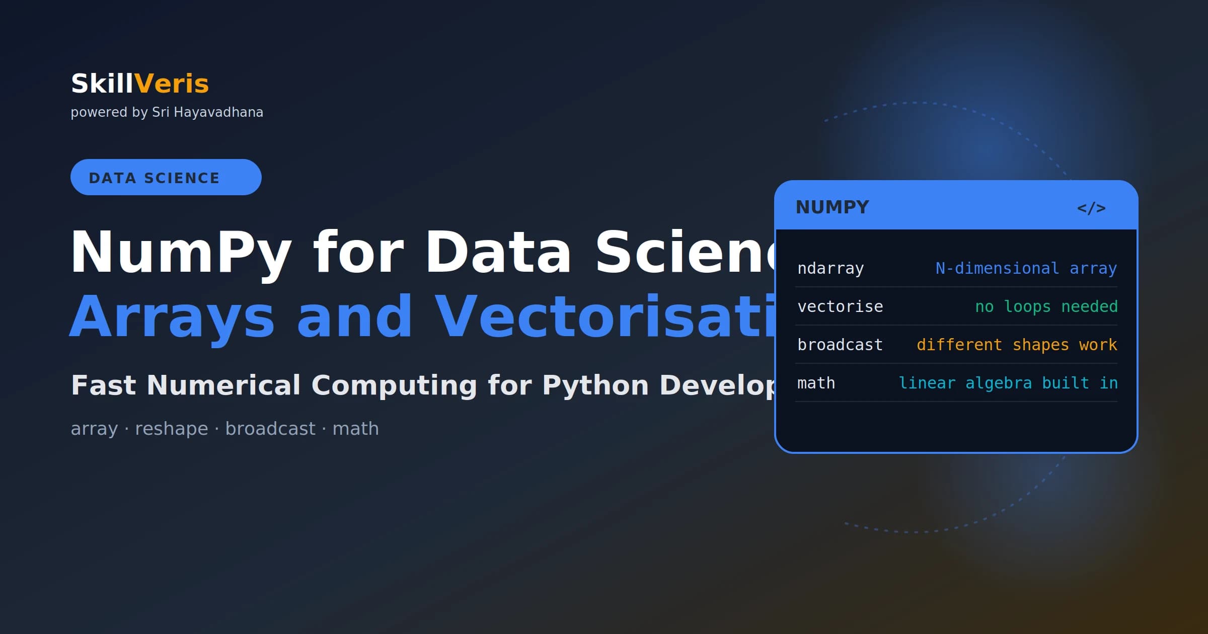
NumPy replaces Python loops with vectorised operations on N-dimensional arrays, running in compiled C for a 10–100x speedup.
In this guide, you'll learn:
- Master array creation, indexing, broadcasting, and universal functions and you have the foundation for pandas, scikit-learn, and PyTorch.
- NumPy slices return views, not copies — use .copy() when you need an independent array.
- Broadcasting automatically aligns array shapes for element-wise operations without explicit loops.
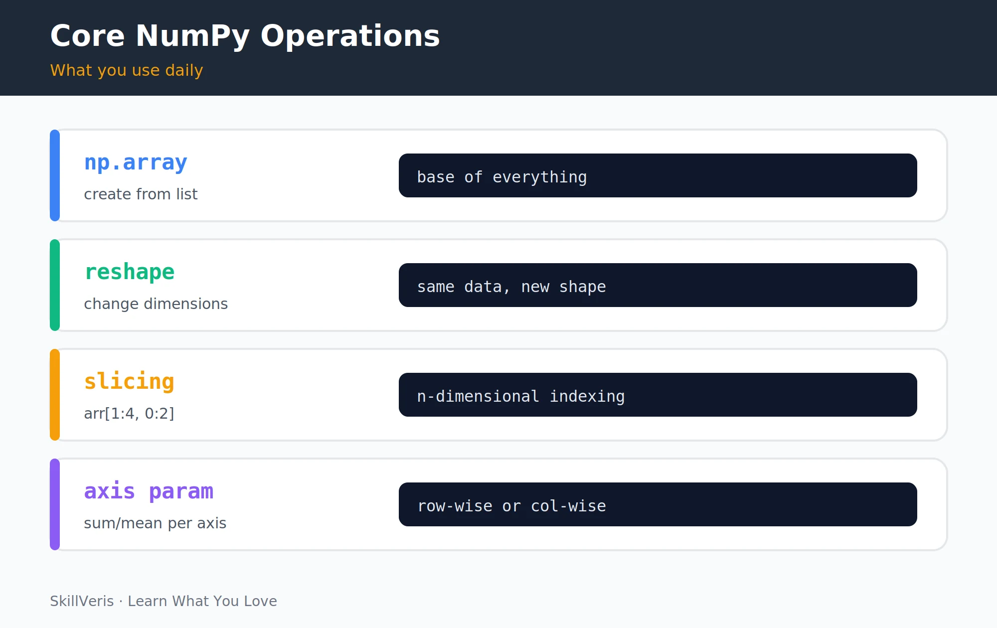
- The axis parameter controls aggregation: axis=0 collapses rows (column results), axis=1 collapses columns (row results).
1What Is NumPy and Why Does It Exist?
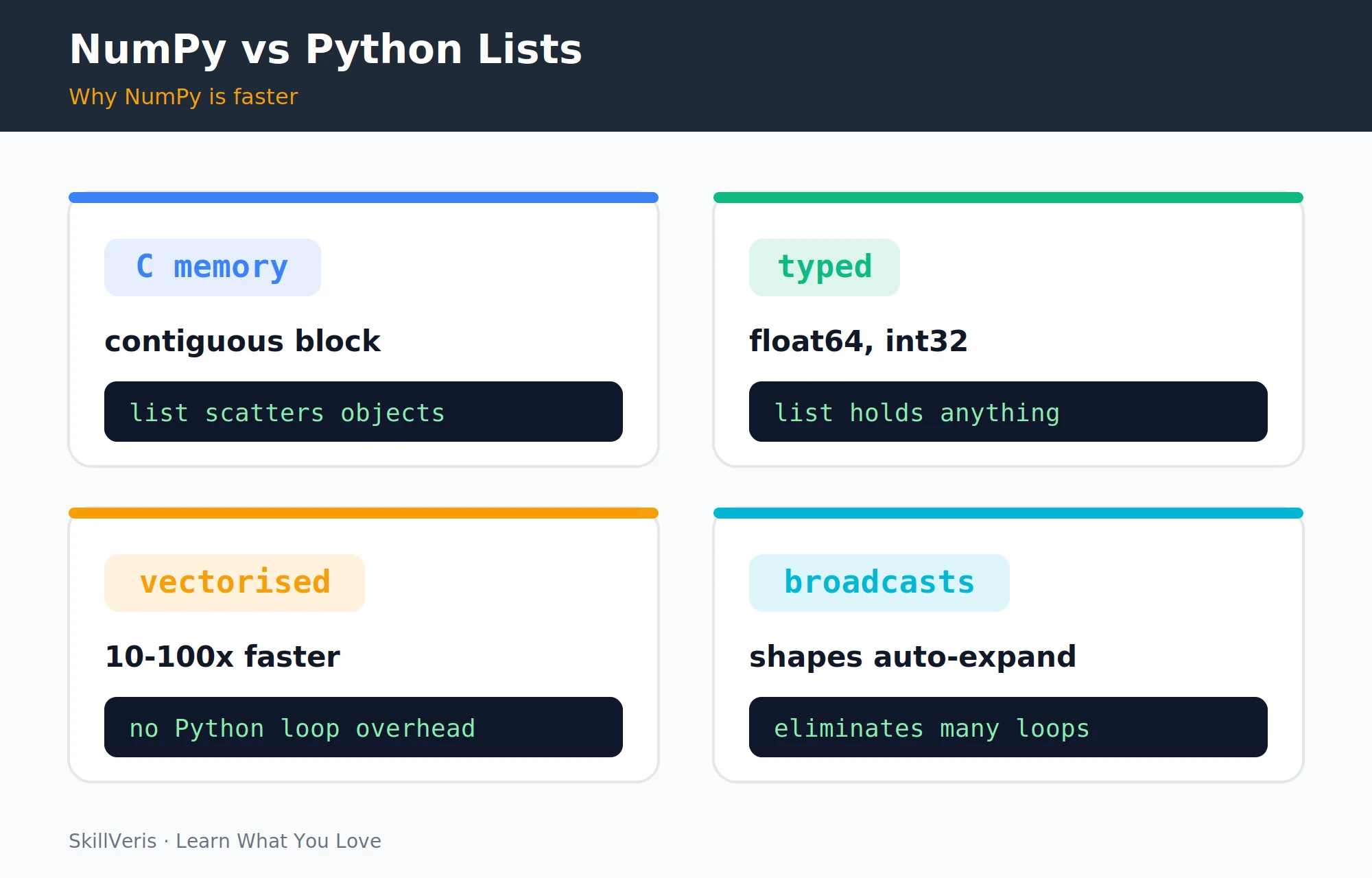
NumPy (Numerical Python) is the foundation of Python's scientific computing ecosystem. Its core object, the ndarray (N-dimensional array), stores elements of the same type in a contiguous block of memory, enabling operations implemented in compiled C rather than interpreted Python. The result is a 10–100x speedup on numerical work compared to Python lists and loops.
Everything in data science uses NumPy underneath: pandas DataFrames are built on ndarrays, scikit-learn operates on them, and PyTorch tensors share the same interface. Understanding NumPy means understanding all of these.
Checking the Version
Import NumPy under its conventional alias.
import numpy as np
print(np.__version__) # 1.26.x or 2.x2Creating Arrays
You can build arrays from Python lists or with built-in constructors for common shapes and ranges. You can also specify the element type with the dtype parameter.
Array Constructors
From lists, ranges, and special matrices, with explicit dtypes.
# From a Python list
a = np.array([1, 2, 3, 4, 5])
# 2D array (matrix)
m = np.array([[1, 2, 3],
              [4, 5, 6]])
# Built-in constructors
np.zeros((3, 4))     # 3x4 matrix of zeros
np.ones((2, 2))      # 2x2 matrix of ones
np.eye(4)            # 4x4 identity matrix
np.arange(0, 10, 2)  # [0, 2, 4, 6, 8]
np.linspace(0, 1, 5) # 5 evenly spaced from 0 to 1
np.random.rand(3, 3) # 3x3 uniform random [0,1)
# Specify dtype
f32 = np.array([1.5, 2.5], dtype=np.float32)
i64 = np.array([1, 2, 3], dtype=np.int64)3Array Properties
Every ndarray exposes attributes describing its shape, dimensionality, size, and memory footprint — useful for debugging shape mismatches.
Inspecting an Array
Shape, dimensions, size, dtype, and byte counts.
a = np.array([[1,2,3],[4,5,6]])
a.shape     # (2, 3) — rows, cols
a.ndim      # 2 — number of dimensions
a.size      # 6 — total number of elements
a.dtype     # dtype('int64')
a.itemsize  # 8 — bytes per element
a.nbytes # 48 — total bytes4Indexing and Slicing
NumPy supports rich indexing: single elements by [row, col], slices across ranges, negative indices, and fancy indexing with lists of positions.
⚠️Watch Out
NumPy slices return views, not copies. Modifying a slice modifies the original array. Use .copy() explicitly when you need an independent array: sub = a[0:2, :].copy().
Indexing a 2D Array
Elements, slices, negative indices, and fancy indexing.
a = np.array([[1,2,3],
              [4,5,6],
              [7,8,9]])
# Single element [row, col]
a[1, 2]      # 6
# Slicing [row_start:end, col_start:end]
a[0:2, 1:3]  # [[2,3],[5,6]]
a[:, 0]      # [1, 4, 7] — first column
a[0, :]      # [1, 2, 3] — first row
# Negative indexing
a[-1, -1]    # 9 — last element
a[-1, :]     # [7, 8, 9] — last row
# Fancy indexing
a[[0, 2], :] # rows 0 and 2: [[1,2,3],[7,8,9]]5Vectorised Operations
Arithmetic and universal functions apply element-wise across an entire array with no Python loop, executing in compiled C. The speed comparison below shows why this matters — NumPy is typically 20–50x faster than the equivalent list comprehension.
Element-wise Math and a Speed Test
Operate on whole arrays at once, then benchmark against a loop.
# Element-wise operations — no loops needed
a = np.array([1, 2, 3, 4])
b = np.array([10, 20, 30, 40])
a + b        # [11, 22, 33, 44]
a * b        # [10, 40, 90, 160]
a ** 2       # [1, 4, 9, 16]
np.sqrt(a)   # [1.0, 1.414, 1.732, 2.0]
np.log(a)    # natural log of each element
np.exp(a)    # e^x for each element
# Speed comparison
import time
n = 1_000_000
lst = list(range(n))
arr = np.arange(n)
start = time.perf_counter()
result_list = [x**2 for x in lst]
print(f"List: {time.perf_counter()-start:.3f}s")
start = time.perf_counter()
result_np = arr**2
print(f"NumPy: {time.perf_counter()-start:.3f}s")
# NumPy is typically 20-50x faster6Broadcasting
Broadcasting lets NumPy perform operations on arrays with different shapes by automatically expanding the smaller array. This is how you add a scalar to every element, add a row vector to each row of a matrix, or standardise columns.
The rules: if shapes differ, prepend 1s to the shorter shape; dimensions of size 1 are stretched to match the other array; and if dimensions are incompatible (neither is 1), NumPy raises an error.
Broadcasting in Practice
Scalars, row vectors, and column-wise standardisation.
# Add a scalar to every element
a = np.array([1, 2, 3])
a + 10  # [11, 12, 13]
# Add a 1D array to each row of a 2D array
m = np.array([[1, 2, 3],
              [4, 5, 6]])
offsets = np.array([10, 20, 30])  # shape (3,)
m + offsets  # [[11,22,33],[14,25,36]] — broadcast across rows
# Standardise each column (subtract mean, divide by std)
data = np.random.randn(100, 5)  # 100 samples, 5 features
mean = data.mean(axis=0)  # shape (5,)
std = data.std(axis=0)    # shape (5,)
standardised = (data - mean) / std # broadcasts across rows7Aggregation Functions
Aggregations like sum, mean, max, and std reduce an array to a summary value. Supply an axis to aggregate along one direction: axis=0 gives column results, axis=1 gives row results. argmax and argmin return the index of the extreme value rather than the value itself.
Aggregating Over Axes
Whole-array reductions and per-axis aggregation.
a = np.array([[1, 2, 3],
              [4, 5, 6]])
# Aggregate over entire array
a.sum()   # 21
a.mean()  # 3.5
a.max()   # 6
a.min()   # 1
a.std()   # standard deviation
# Aggregate along an axis
a.sum(axis=0)   # column sums: [5, 7, 9]
a.sum(axis=1)   # row sums: [6, 15]
a.max(axis=1)   # row maxima: [3, 6]
a.mean(axis=0)  # column means: [2.5, 3.5, 4.5]
# argmax/argmin: index of max/min
a.argmax()        # 5 (flat index)
a.argmax(axis=0) # [1, 1, 1] — row index of max in each column8Reshaping and Stacking
reshape gives the same data a new shape, and -1 lets NumPy infer one dimension. ravel returns a view while flatten returns a copy. np.newaxis adds a dimension (common for ML model inputs), and vstack/hstack combine arrays.
Changing Shape and Combining Arrays
Reshape, flatten, add dimensions, and stack.
# Reshape: same data, different dimensions
a = np.arange(12)        # [0..11] shape (12,)
m = a.reshape(3, 4)      # shape (3, 4)
t = a.reshape(2, 2, 3)   # shape (2, 2, 3)
f = a.reshape(-1, 3)     # -1 = infer: shape (4, 3)
# Flatten back to 1D
m.ravel()    # view (no copy)
m.flatten()  # copy
# Add a dimension (common for ML model inputs)
a = np.array([1, 2, 3])  # shape (3,)
a[np.newaxis, :]  # shape (1, 3) — row vector
a[:, np.newaxis]  # shape (3, 1) — column vector
# Stacking
x = np.array([1, 2, 3])
y = np.array([4, 5, 6])
np.vstack([x, y])  # [[1,2,3],[4,5,6]] — stack as rows
np.hstack([x, y]) # [1,2,3,4,5,6] — concatenate horizontally9Boolean Indexing
Boolean masks select elements meeting a condition, combine conditions with & and |, and drive conditional replacement with np.where. np.clip bounds values to a range, and np.where with a single argument returns the indices of matching elements.
Filtering and Conditional Replacement
Select, combine conditions, replace, clip, and locate.
# Select elements meeting a condition
a = np.array([3, -1, 4, -2, 5])
positives = a[a > 0]   # [3, 4, 5]
# Multiple conditions
a[(a > 0) & (a < 5)]   # [3, 4]
# Where: conditional replacement
np.where(a > 0, a, 0)  # [3, 0, 4, 0, 5] — replace negatives with 0
# Clip values to a range
np.clip(a, 0, 4)       # [3, 0, 4, 0, 4]
# Find indices of matching elements
np.where(a > 0) # (array([0, 2, 4]),)10Linear Algebra
NumPy's linalg module covers the linear algebra you need: matrix products with @, determinants, inverses, solving linear systems, eigendecomposition, and vector norms. Note that @ is matrix multiplication while * is element-wise.
linalg Operations
Matrix products and common decompositions.
from numpy import linalg
A = np.array([[2, 1], [1, 3]])
b = np.array([5, 10])
# Matrix multiplication
A @ A  # matrix product (same as np.matmul(A, A))
A * A  # element-wise product (NOT matrix mult)
# Linear algebra operations
linalg.det(A)      # determinant: 5.0
linalg.inv(A)      # inverse matrix
linalg.solve(A, b) # solve Ax=b: [1.0, 3.0]
linalg.eig(A)      # eigenvalues and eigenvectors
linalg.norm(b) # L2 norm of vector b11Random Number Generation
Prefer the modern default_rng API (NumPy 1.17+), which gives a reproducible generator when seeded. From it you can draw uniform, integer, and normal samples, make random choices, and shuffle arrays in place.
The Modern Generator API
Seed for reproducibility, then sample and shuffle.
# Modern API (NumPy 1.17+) — prefer this
rng = np.random.default_rng(seed=42)  # reproducible
rng.random((3, 3))           # uniform [0, 1)
rng.integers(0, 100, 10)     # 10 random ints 0-99
rng.normal(0, 1, (5, 5))     # normal distribution
rng.choice(["a","b","c"], 10) # random sampling
# Shuffle an array in-place
arr = np.arange(10)
rng.shuffle(arr)12Key Takeaways
NumPy is the bedrock of the Python data stack — these are the ideas that carry over everywhere.
- NumPy's ndarray is a typed, contiguous-memory array enabling vectorised C operations — 10–100x faster than Python loops.
- Slices return views (not copies); use .copy() when you need independence.
- Broadcasting automatically aligns array shapes for element-wise operations without explicit loops.
- The axis parameter controls aggregation: axis=0 collapses rows (column results), axis=1 collapses columns (row results).
- All of pandas, scikit-learn, and PyTorch build on NumPy ndarrays; learning NumPy makes everything else easier.
13What to Learn Next
Build on NumPy with the libraries that depend on it.
- Pandas for Beginners — DataFrames are built on NumPy arrays.
- Machine Learning for Beginners — scikit-learn uses NumPy arrays as input.
- Data Visualisation Best Practices — matplotlib plots NumPy arrays directly.
14Frequently Asked Questions
Why is @ used for matrix multiplication in NumPy? The @ operator (introduced in Python 3.5 via PEP 465) is the matrix multiplication operator. A @ B computes the dot product (matrix multiplication); A * B computes element-wise multiplication. Always use @ for matrix products — it's clearer than np.dot() and avoids the ambiguity of *.
What is the difference between np.arange and np.linspace? np.arange(start, stop, step) creates an array with a fixed step size (like Python's range()). np.linspace(start, stop, n) creates an array with a fixed number of elements, evenly spaced between start and stop (inclusive). Use linspace when you want a specific number of points; use arange when you want a specific step.
When should I use NumPy vs pandas? NumPy is for homogeneous numerical arrays, mathematical operations, and anything that needs raw speed. Pandas is for heterogeneous tabular data (mixed types, string column names, time series). In practice: load data with pandas, extract numerical columns as NumPy arrays for heavy computation, then put results back into a DataFrame.
Is NumPy enough for machine learning, or do I need PyTorch/TensorFlow? NumPy is enough to implement classical ML algorithms (linear regression, k-nearest neighbours, decision trees) from scratch — excellent for learning. For production deep learning (neural networks, GPUs, automatic differentiation), you need PyTorch or TensorFlow. Think of NumPy as the foundation and PyTorch as the skyscraper built on it.
Related Reading
Get The Print Version
Download a PDF of this article for offline reading.
About the Publisher
SkillVeris Team
Data Science Team
Our data team shares real-world analytics, ML, and SQL insights grounded in industry practice.
View all postsRelated Posts
Never miss an update
Get the latest tutorials and guides delivered to your inbox.
No spam. Unsubscribe anytime.