SQL Tutorial for Beginners: With Real Examples
SkillVeris Team
Engineering Team
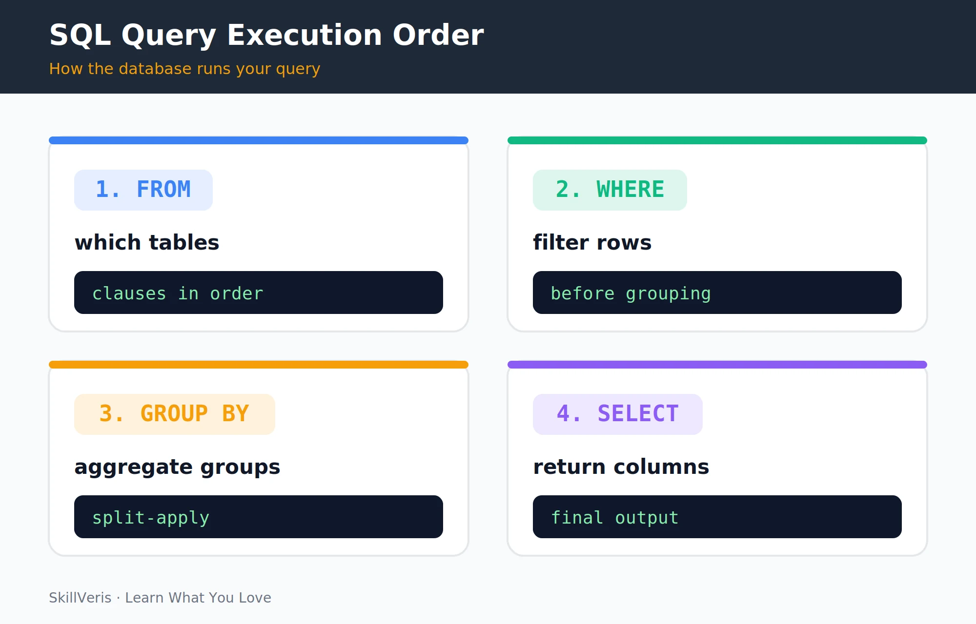
SQL queries follow a logical order: FROM, WHERE, GROUP BY, HAVING, SELECT, ORDER BY.
In this guide, you'll learn:
- Master those six clauses and you can answer almost any data question from a relational database.
- WHERE filters rows before grouping, while HAVING filters groups after aggregation.
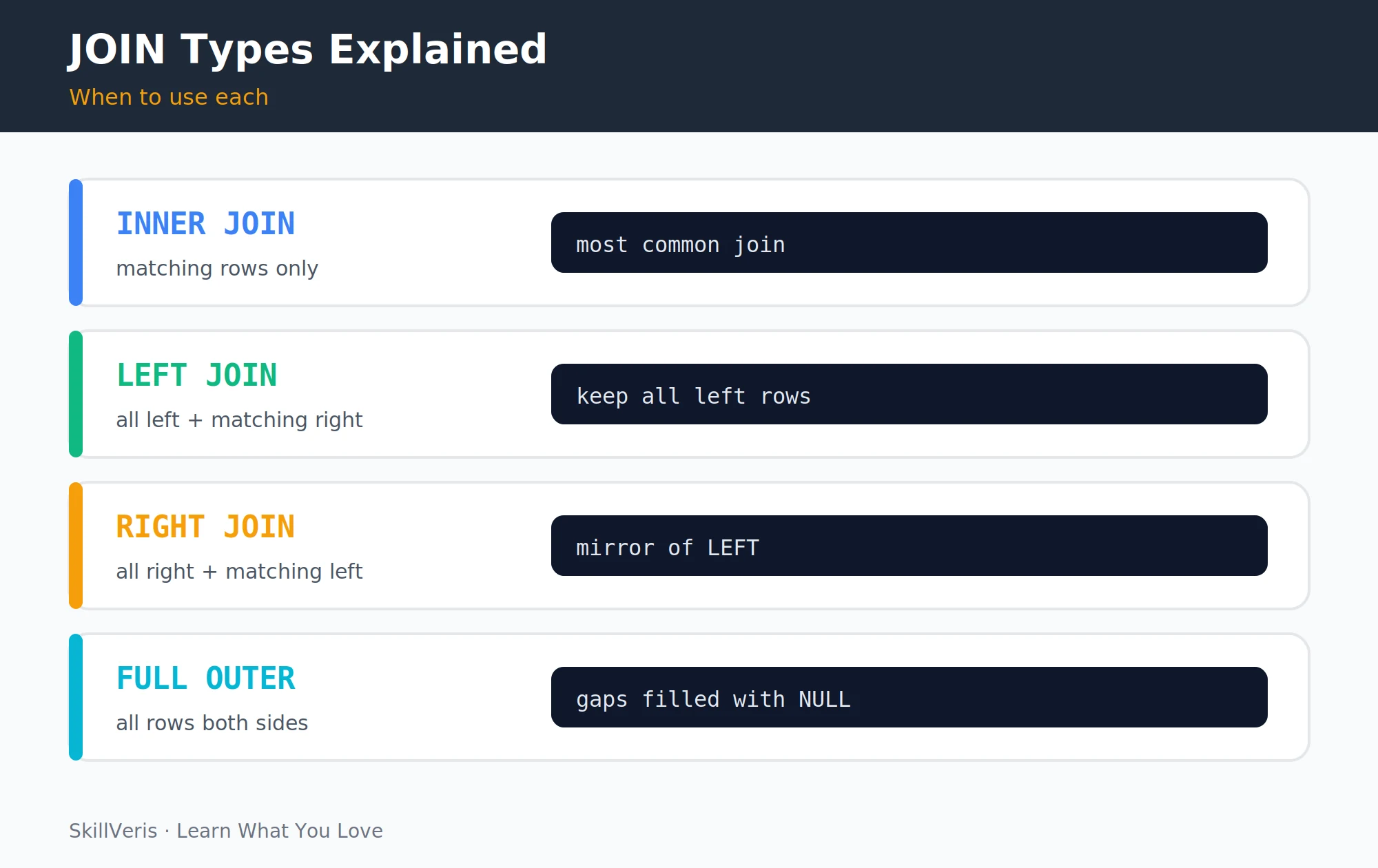
- INNER JOIN keeps only matching rows; LEFT JOIN keeps every row from the left table.
- CTEs (WITH clauses) name intermediate results and make complex queries far more readable.
1What Is SQL and Why Learn It?
SQL (Structured Query Language) is the standard language for querying relational databases. Every major data store — PostgreSQL, MySQL, SQLite, BigQuery, Snowflake, Redshift — speaks SQL.
Data analysts use it to extract insights, backend developers use it to build applications, and data scientists use it to explore datasets before modelling. It consistently appears at the top of "most useful skills" lists for data roles.
2Setting Up: SQLite
SQLite requires no server installation — it runs entirely from a file and is built into Python. You can create an in-memory database, set up sample tables, and start querying in a few lines.
Alternatively, install DB Browser for SQLite for a free visual query editor if you prefer a graphical interface.
Create sample tables
Seed an in-memory database:
import sqlite3

# Create in-memory database (or use "company.db" for a file)
conn = sqlite3.connect(":memory:")
cursor = conn.cursor()

# Create sample tables
cursor.executescript(
    "CREATE TABLE employees (id INTEGER PRIMARY KEY, name TEXT, dept TEXT, salary REAL, hire_year INTEGER);"
    "INSERT INTO employees VALUES (1,'Alice','Engineering',95000,2020),"
    "(2,'Bob','Engineering',88000,2019),(3,'Carol','Marketing',72000,2021),"
    "(4,'Dave','Marketing',68000,2022),(5,'Eve','Engineering',102000,2018);"
    "CREATE TABLE projects (id INTEGER PRIMARY KEY, name TEXT, dept TEXT, budget REAL);"
    "INSERT INTO projects VALUES (1,'Alpha','Engineering',500000),(2,'Beta','Marketing',120000),(3,'Gamma','Engineering',350000);"
)
conn.commit()
print("Database ready")3SELECT and FROM
SELECT chooses which columns to return and FROM names the table. You can select all columns with *, pick specific columns, rename them with aliases, or remove duplicates with DISTINCT.
Understanding execution order — FROM runs before SELECT — prevents common mistakes later, especially with WHERE versus HAVING.
SELECT basics
Columns, aliases, and DISTINCT:
-- Select all columns
SELECT * FROM employees;

-- Select specific columns
SELECT name, dept, salary FROM employees;

-- Column aliases
SELECT name AS employee_name,
       salary / 12 AS monthly_salary
FROM employees;

-- Remove duplicates
SELECT DISTINCT dept FROM employees;4WHERE: Filtering Rows
WHERE filters individual rows before any grouping happens. It supports comparison operators, AND/OR logic, IN for sets, BETWEEN for ranges, LIKE for pattern matching, and IS NULL / IS NOT NULL for null checks.
Combining these conditions lets you express almost any row-level filter you need.
Filtering conditions
Comparisons, IN, BETWEEN, LIKE, and NULL:
-- Simple condition
SELECT * FROM employees WHERE salary > 90000;

-- Multiple conditions
SELECT * FROM employees
WHERE dept = 'Engineering' AND salary > 90000;

-- OR condition
SELECT name FROM employees
WHERE dept = 'Marketing' OR hire_year < 2020;

-- IN: match one of many values
SELECT * FROM employees
WHERE dept IN ('Engineering', 'Data');

-- BETWEEN (inclusive)
SELECT name, salary FROM employees
WHERE salary BETWEEN 70000 AND 100000;

-- LIKE: pattern matching
SELECT * FROM employees WHERE name LIKE 'A%';  -- starts with A
SELECT * FROM employees WHERE name LIKE '%e';  -- ends with e

-- NULL checks
SELECT * FROM employees WHERE dept IS NOT NULL;5ORDER BY and LIMIT
ORDER BY sorts the result set, ascending by default or descending with DESC, and you can sort by multiple columns. LIMIT caps the number of rows returned, and OFFSET skips rows for pagination.
Combining ORDER BY with LIMIT is the standard way to fetch top-N rows, such as the highest earners.
Sorting and paging
Order, limit, and paginate:
-- Sort ascending (default)
SELECT name, salary FROM employees ORDER BY salary;

-- Sort descending
SELECT name, salary FROM employees ORDER BY salary DESC;

-- Multi-column sort
SELECT * FROM employees
ORDER BY dept ASC, salary DESC;

-- Top N rows
SELECT name, salary
FROM employees
ORDER BY salary DESC
LIMIT 3;  -- top 3 earners

-- Pagination
SELECT * FROM employees
ORDER BY id
LIMIT 10 OFFSET 20; -- rows 21-306Aggregate Functions
Aggregate functions collapse many rows into a single value: COUNT, SUM, AVG, MAX, and MIN. They ignore NULLs, except COUNT(*) which counts all rows including those with NULLs.
Combining several aggregates in one SELECT gives you a quick statistical summary of a table.
💡Pro Tip
Use COUNT(DISTINCT column) to count unique values — invaluable for "how many unique customers placed orders?" type questions. It's a very common interview question pattern.
Summary statistics
Count, sum, average, max, and min:
SELECT
  COUNT(*) AS total_employees,
  COUNT(DISTINCT dept) AS departments,
  SUM(salary) AS total_payroll,
  AVG(salary) AS avg_salary,
  MAX(salary) AS highest_salary,
  MIN(salary) AS lowest_salary
FROM employees;7GROUP BY
GROUP BY splits rows into groups so aggregates apply per group rather than across the whole table — for example, headcount and average salary per department. You can group by multiple columns to break the data down further.
Rule: every column in SELECT that is not inside an aggregate function must appear in GROUP BY. This is the most common GROUP BY error.
Grouping rows
Aggregate per group:
-- Employee count and average salary per department
SELECT
  dept,
  COUNT(*) AS headcount,
  AVG(salary) AS avg_salary,
  SUM(salary) AS total_salary
FROM employees
GROUP BY dept
ORDER BY avg_salary DESC;

-- Group by multiple columns
SELECT dept, hire_year, COUNT(*) AS hires
FROM employees
GROUP BY dept, hire_year
ORDER BY dept, hire_year;8HAVING: Filter After Grouping
HAVING filters groups after aggregation, which is what you need when the condition involves an aggregate value such as an average or a count. You cannot use aggregate functions in WHERE.
The key distinction: WHERE filters rows before grouping, while HAVING filters the grouped results afterward.
Filtering groups
Conditions on aggregates:
-- Departments with avg salary > 80,000
SELECT dept, AVG(salary) AS avg_sal
FROM employees
GROUP BY dept
HAVING AVG(salary) > 80000;

-- Departments with more than 2 employees
SELECT dept, COUNT(*) AS n
FROM employees
GROUP BY dept
HAVING COUNT(*) > 2;9Joins: Combining Tables
Joins combine rows from two tables based on a matching condition. INNER JOIN returns only rows that match in both tables, while LEFT JOIN returns all rows from the left table with NULLs where there's no match.
A self-join joins a table to itself, which is useful for comparing rows within the same table.
Join types
Inner, left, and self-joins:
-- INNER JOIN: only rows that match in both tables
SELECT e.name, e.dept, p.name AS project
FROM employees e
JOIN projects p ON e.dept = p.dept;

-- LEFT JOIN: all employees, project info where available
SELECT e.name, p.name AS project
FROM employees e
LEFT JOIN projects p ON e.dept = p.dept;
-- employees without a project show NULL for p.name

-- Self-join: compare rows within same table
SELECT a.name, b.name, a.dept
FROM employees a
JOIN employees b ON a.dept = b.dept AND a.id < b.id;10Subqueries
A subquery is a query nested inside another, useful for comparing against a computed value such as the company-wide average salary. Subqueries can also act as derived tables in the FROM clause.
Common Table Expressions (CTEs), written with a WITH clause, name an intermediate result and are cleaner than deeply nested subqueries.
Subqueries and CTEs
Inline, derived table, and WITH:
-- Employees earning above company average
SELECT name, salary
FROM employees
WHERE salary > (
    SELECT AVG(salary) FROM employees
);

-- Using a subquery as a derived table
SELECT dept, avg_sal
FROM (SELECT dept, AVG(salary) AS avg_sal
      FROM employees
      GROUP BY dept) AS dept_avg
WHERE avg_sal > 80000;

-- CTEs (Common Table Expressions) -- cleaner than nested subqueries
WITH dept_avg AS (
    SELECT dept, AVG(salary) AS avg_sal
    FROM employees
    GROUP BY dept
)
SELECT e.name, e.salary, d.avg_sal
FROM employees e
JOIN dept_avg d ON e.dept = d.dept
WHERE e.salary > d.avg_sal;11Window Functions
Window functions apply an aggregation or ranking to a set of rows (the "window") without collapsing them — so unlike GROUP BY, all original rows remain in the output. RANK, running SUM, and LAG are common examples.
They're one of the most powerful SQL features and appear constantly in data analyst technical interviews.
Ranking and running totals
RANK, running SUM, and LAG:
-- Rank employees by salary within their department
SELECT
  name, dept, salary,
  RANK() OVER (
    PARTITION BY dept
    ORDER BY salary DESC
  ) AS dept_rank,
  AVG(salary) OVER (PARTITION BY dept) AS dept_avg
FROM employees;

-- Running total of payroll (ordered by hire year)
SELECT
  name, hire_year, salary,
  SUM(salary) OVER (ORDER BY hire_year) AS running_payroll
FROM employees;

-- Compare each employee's salary to previous hire's salary
SELECT
  name, hire_year, salary,
  LAG(salary) OVER (ORDER BY hire_year) AS prev_hire_salary
FROM employees;12Key Takeaways
A few core ideas underpin almost every SQL query you'll write, from filtering to joining to ranking.
- Execution order: FROM -> WHERE -> GROUP BY -> HAVING -> SELECT -> ORDER BY -> LIMIT.
- WHERE filters rows before grouping; HAVING filters groups after aggregation.
- INNER JOIN keeps only matching rows; LEFT JOIN keeps all rows from the left table.
- CTEs (WITH name AS (...)) make complex queries readable by naming intermediate results.
- Window functions aggregate without collapsing rows — essential for rankings and running totals.
13What to Learn Next
Reinforce these techniques by applying them to real data and connecting SQL to the wider data stack.
- Learn SQL Through Football Data — apply these techniques to real sports data.
- Data Analytics Roadmap — SQL is step one in the full path.
- Build a REST API with FastAPI — use SQLAlchemy to run SQL from Python.
14Frequently Asked Questions
What is the difference between SQL and NoSQL? SQL databases like PostgreSQL, MySQL, and SQLite store data in structured tables with fixed schemas and use SQL for queries. NoSQL databases like MongoDB, Cassandra, and Redis use flexible schemas and their own query languages. SQL is better for structured, relational data with complex queries; NoSQL suits unstructured data, high write throughput, or simple key-value lookups.
Which SQL database should I learn on? Start with SQLite for learning since it needs no setup and runs in Python, then move to PostgreSQL for production and most job roles. MySQL is common in web development. The SQL you learn in one transfers to all others with minor syntax differences.
How is a CTE different from a subquery? Both produce a temporary result set. CTEs (WITH clauses) are defined at the top and referenced by name, making complex queries much more readable, and they can also be recursive for hierarchical data. Subqueries are nested inline. Prefer CTEs for readability when a subquery would be deeply nested.
Do I need to know SQL if I use pandas? Yes. Most real data lives in databases, and SQL is the standard way to extract it before loading it into pandas. SQL also scales to datasets too large for pandas. The two skills complement each other: SQL to extract and aggregate, pandas to transform and analyse.
Related Reading
Get The Print Version
Download a PDF of this article for offline reading.
About the Publisher
SkillVeris Team
Engineering Team
Our engineering writers turn abstract code concepts into hands-on, project-driven learning experiences.
View all postsRelated Posts

Never miss an update
Get the latest tutorials and guides delivered to your inbox.
No spam. Unsubscribe anytime.